Generating Synthetic MMM Data

Before trusting a Media Mix Model (MMM) on real business data, we need confidence that it can actually recover the parameters that generated the observations. Parameter recovery is the gold-standard validation technique: we generate synthetic data from known ground-truth values, fit the model back on that data, and check whether the posteriors concentrate around the true values. See for example the MMM Example Notebook notebook as a practical example of parameter recovery.

This notebook walks through the full parameter recovery workflow:

1. Generate correlated channel spend covariates using a multivariate normal model with an LKJ prior on the correlation structure.

2. Fix known “true” parameter values for adstock, saturation, seasonality, and noise.

3. Forward-sample through the MMM using PyMC’s do operator to produce a synthetic observed target variable.

4. Fit the MMM on the synthetic data using the same model specification.

5. Verify recovery by comparing posterior distributions against the ground-truth values.

We use pymc-marketing’s MMM class with GeometricAdstock and LogisticSaturation transformations, and rely on PyMC’s do operator for causal intervention (clamping parameters to their true values during data generation).

Prepare Notebook

import arviz as az
import matplotlib.pyplot as plt
import numpy as np
import pandas as pd
import pymc as pm
import pytensor.tensor as pt
import seaborn as sns
from pymc import do
from pymc_extras.prior import Prior

from pymc_marketing.mmm import GeometricAdstock, LogisticSaturation
from pymc_marketing.mmm.multidimensional import MMM

az.style.use("arviz-darkgrid")
plt.rcParams["figure.figsize"] = [10, 6]
plt.rcParams["figure.dpi"] = 100
plt.rcParams["figure.facecolor"] = "white"

%load_ext autoreload
%autoreload 2
%config InlineBackend.figure_format = "retina"

seed: int = sum(map(ord, "mmm"))
rng: np.random.Generator = np.random.default_rng(seed=seed)

Generating Covariates Data

The first step is to generate realistic media channel spend data. Real-world channel spends are typically correlated (e.g., brands may increase spend across multiple channels simultaneously during campaigns) and exhibit trends over time. We model this with a PyMC generative model that captures both properties.

# Configuration Parameters

n_dates = 120

date_range = pd.date_range(start="2020-01-01", freq="W-MON", periods=n_dates)


n_channels = 5

l_max = 6

n_fourier_modes = 3

chol_eta = 3

coords = {"channel": [f"x{i}" for i in range(n_channels)], "date": date_range}

Generative model for covariates:

We build a PyMC model where each channel’s spend at each time step is drawn from a multivariate normal distribution:

• Time normalization: t is scaled to \([0, 1)\) so the linear trend coefficients are on a comparable scale.

• LKJ Cholesky prior (LKJCholeskyCov): Induces a realistic correlation structure across channels. The Cholesky factor L is used directly in the MvNormal likelihood for numerical stability.

• Linear trends: Each channel gets its own intercept a and slope b, so channels can have different baseline levels and growth/decline trajectories over time.

• Multivariate normal draws: At each time step the 5-dimensional channel vector is drawn from MvNormal(mu, chol=L), ensuring cross-channel correlations.

• Softplus transformation: softplus(x) = log(1 + exp(x)) ensures all spend values are non-negative, which is a hard constraint for media spend data.

Tip

Depending on your industry, you may need to use a different data generation process.

t = np.arange(n_dates) / n_dates

with pm.Model(coords=coords) as covariates_model:
    t_data = pm.Data("t", t, dims=("date",))

    L, _, _ = pm.LKJCholeskyCov(
        "L",
        n=len(coords["channel"]),
        eta=chol_eta,
        sd_dist=pm.Exponential.dist(lam=1 / 3),
    )

    a = pm.Normal("a", mu=0, sigma=1, dims="channel")
    b = pm.Normal("b", mu=0, sigma=1, dims="channel")

    mu = pm.Deterministic("mu", a + b * t_data[..., None], dims=("date", "channel"))

    x_raw = pm.MvNormal("x_raw", mu=mu, chol=L, dims=("date", "channel"))

    x = pm.Deterministic("x", pt.softplus(x_raw), dims=("date", "channel"))

pm.model_to_graphviz(covariates_model)

We draw a single realization from the covariates model and assemble it into a pandas DataFrame. A dummy target column y_dummy = 1 is added as a placeholder; it will be replaced later with the actual synthetic observations.

x_data = pm.draw(covariates_model.x, draws=1, random_seed=rng)

mmm_df = pd.DataFrame(x_data, columns=coords["channel"]).assign(
    date=date_range, y_dummy=np.ones(n_dates)
)

col = mmm_df.pop("date")
mmm_df.insert(0, "date", col)

mmm_df.head()

	date	x0	x1	x2	x3	x4	y_dummy
0	2020-01-06	6.208217	1.239197	0.455048	3.493189	0.997002	1.0
1	2020-01-13	3.640003	0.096297	0.744953	0.366538	2.316299	1.0
2	2020-01-20	5.412316	0.012111	0.133368	5.640305	2.368558	1.0
3	2020-01-27	0.167504	0.689889	1.906349	0.278028	0.518104	1.0
4	2020-02-03	0.025429	0.289182	0.750129	0.013511	1.466233	1.0

Specify Model Configuration

Now we draw the ground-truth parameter values from some distributions. We do not use a single value as we would want to wrap this code into functions to generate many datasets with different parameter values. After that we define the mmm_generator object that will be used to generate the synthetic data.

intercept_true = pm.draw(pm.Normal.dist(sigma=2), draws=1, random_seed=rng)
adstock_alpha_true = pm.draw(
    pm.Beta.dist(alpha=1, beta=3), draws=len(coords["channel"]), random_seed=rng
)
saturation_beta_true = pm.draw(
    pm.HalfNormal.dist(sigma=2), draws=len(coords["channel"]), random_seed=rng
)
saturation_lam_true = pm.draw(
    pm.Gamma.dist(alpha=2, beta=1), draws=len(coords["channel"]), random_seed=rng
)
gamma_fourier_true = pm.draw(
    pm.Laplace.dist(mu=0, b=0.2, size=2 * n_fourier_modes), random_seed=rng
)
y_sigma_true = pm.draw(pm.HalfNormal.dist(sigma=3), draws=1, random_seed=rng)


model_config = {
    "intercept": Prior("Normal", mu=0, sigma=2),
    "adstock_alpha": Prior("Beta", alpha=1, beta=3, dims="channel"),
    "saturation_beta": Prior("HalfNormal", sigma=2, dims="channel"),
    "saturation_lam": Prior("Gamma", alpha=2, beta=1, dims="channel"),
    "gamma_control": Prior("Normal", mu=0, sigma=1, dims="control"),
    "gamma_fourier": Prior("Laplace", mu=0, b=0.2, dims="fourier_mode"),
    "likelihood": Prior("Normal", sigma=Prior("HalfNormal", sigma=3)),
}

mmm_generator = MMM(
    date_column="date",
    target_column="y_dummy",
    channel_columns=coords["channel"],
    adstock=GeometricAdstock(l_max=l_max),
    saturation=LogisticSaturation(),
    yearly_seasonality=n_fourier_modes,
    model_config=model_config,
)

Generate Target Variable

Now we use the MMM’s generative structure to produce synthetic observations. The strategy is a forward simulation through the model graph with the parameters clamped to their known true values:

1. Build the model graph: mmm_generator.build_model(X, y_dummy) compiles the full MMM computation graph. We also register original-scale contribution variables (before target scaling) so we can inspect the true decomposition later.

2. Intervene with do: PyMC’s do operator clamps stochastic nodes to their ground-truth values. This turns the probabilistic model into a deterministic forward simulator (aside from observation noise \(\sigma\)), ensuring the synthetic data is generated from exactly the parameter values we want to recover.

3. Sample forward: pm.sample_prior_predictive(draws=1) propagates the clamped values through the adstock, saturation, and seasonality transformations to produce one synthetic target time series.

4. Assemble final data: The synthetic y_obs replaces the dummy target. We drop the first l_max rows because the geometric adstock transformation needs a burn-in window to avoid edge effects.

X = mmm_df.drop(columns=["y_dummy"])
y_dummy = mmm_df["y_dummy"]

mmm_generator.build_model(X, y_dummy)
mmm_generator.add_original_scale_contribution_variable(
    var=[
        "channel_contribution",
        "intercept_contribution",
        "yearly_seasonality_contribution",
        "y",
    ]
)

mmm_generator.model = do(
    mmm_generator.model,
    {
        "intercept_contribution": intercept_true,
        "adstock_alpha": adstock_alpha_true,
        "saturation_beta": saturation_beta_true,
        "saturation_lam": saturation_lam_true,
        "gamma_fourier": gamma_fourier_true,
        "y_sigma": y_sigma_true,
    },
)

with mmm_generator.model:
    idata_obs = pm.sample_prior_predictive(
        draws=1,
        var_names=[
            "y",
            "y_original_scale",
            "channel_contribution_original_scale",
        ],
        random_seed=rng,
    )

Sampling: [y]

y_obs = idata_obs["prior"]["y_original_scale"].sel(chain=0, draw=0)

mmm_df["y_obs"] = y_obs

# Remove last dates (adstock lag)
mmm_df = mmm_df.tail(-l_max)
coords["date"] = coords["date"][l_max:]

mmm_df.head()

	date	x0	x1	x2	x3	x4	y_dummy	y_obs
6	2020-02-17	4.364082	1.958480	1.873190	0.005611	0.804895	1.0	2.381511
7	2020-02-24	0.735180	1.442319	0.682221	5.882805	0.572488	1.0	0.886471
8	2020-03-02	7.069741	0.560737	0.417488	0.001453	0.217027	1.0	0.855292
9	2020-03-09	0.312553	0.208669	0.106582	0.001532	1.392096	1.0	-0.278851
10	2020-03-16	1.582743	0.026846	0.065228	0.025798	1.817333	1.0	-0.255760

Exploratory Visualizations

Before moving to parameter recovery, we inspect the synthetic data to confirm it looks reasonable:

mmm_df[coords["channel"]].corr()

	x0	x1	x2	x3	x4
x0	1.000000	-0.117607	-0.070978	-0.176938	0.212297
x1	-0.117607	1.000000	0.027311	0.017998	-0.501167
x2	-0.070978	0.027311	1.000000	0.046590	0.039386
x3	-0.176938	0.017998	0.046590	1.000000	0.145880
x4	0.212297	-0.501167	0.039386	0.145880	1.000000

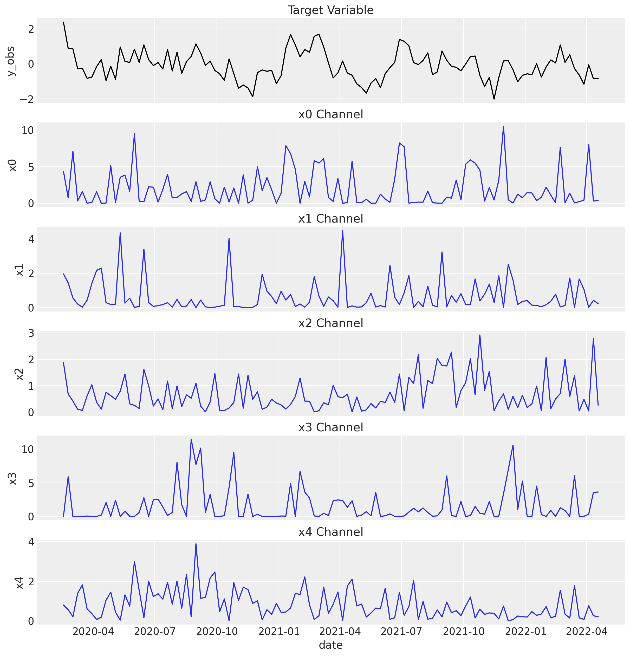
Let’s look at the target variable and each channel’s spend over time.

fig, ax = plt.subplots(
    nrows=len(coords["channel"]) + 1,
    figsize=(12, len(coords["channel"]) * 2.5),
    sharex=True,
)

sns.lineplot(x="date", y="y_obs", data=mmm_df, color="black", ax=ax[0])
ax[0].set_title("Target Variable")

for i, channel in enumerate(coords["channel"]):
    sns.lineplot(x="date", y=channel, data=mmm_df, color="C0", ax=ax[i + 1])
    ax[i + 1].set_title(f"{channel} Channel")

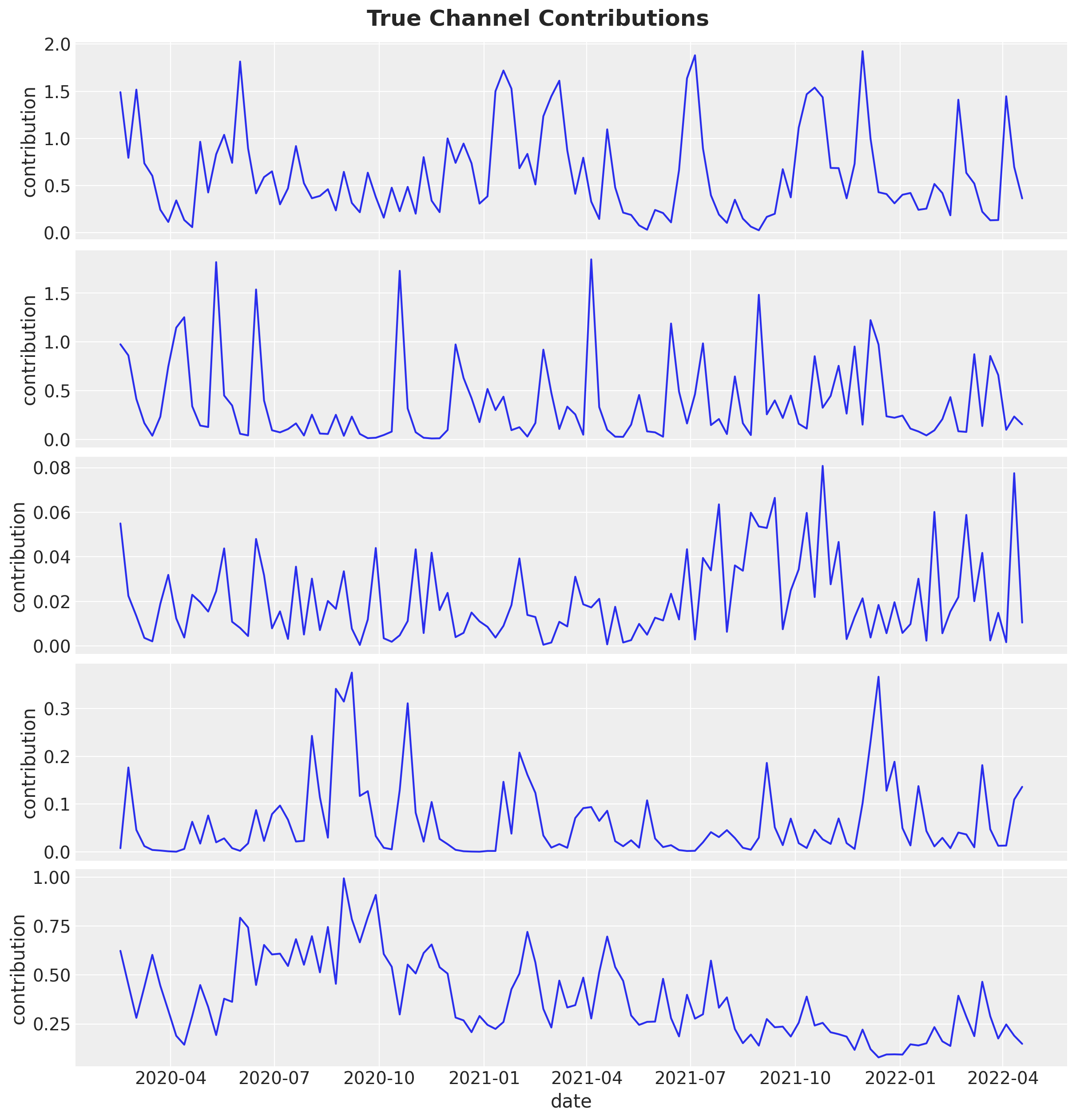
Now, we plot the true channel contributions from the generative model.

fig, axes = plt.subplots(
    nrows=len(coords["channel"]),
    figsize=(12, len(coords["channel"]) * 2.5),
    sharex=True,
)

for i, channel in enumerate(coords["channel"]):
    channel_contribution_observed = (
        idata_obs["prior"]["channel_contribution_original_scale"]
        .sel(chain=0, draw=0)
        .sel(channel=channel)
        .to_numpy()[l_max:]
    )

    sns.lineplot(
        data=mmm_df, x="date", y=channel_contribution_observed, color="C0", ax=axes[i]
    )

    axes[i].set(ylabel="contribution")

fig.suptitle("True Channel Contributions", fontsize=18, fontweight="bold");

Parameter Recovery

With the synthetic data in hand, we now fit the MMM and check whether the posteriors recover the true parameter values. This is the core validation step: if the model cannot recover known parameters from clean synthetic data, we should not trust it on noisy real-world data.

Fit Model

We create a new MMM instance that targets y_obs (the synthetic data) and fit it using MCMC.

Informative priors via channel shares: Before fitting, we adjust the saturation_beta prior. The sigma of the HalfNormal prior is scaled by each channel’s share of total spend (n_channels * channel_shares), encoding the reasonable belief that channels with more spend are likely to have larger effect magnitudes. This is a common practice that helps the sampler explore more efficiently.

channel_shares = (
    mmm_df[coords["channel"]].sum(axis=0) / mmm_df[coords["channel"]].sum(axis=0).sum()
).to_numpy()

prior_sigma = n_channels * channel_shares

model_config["saturation_beta"] = Prior("HalfNormal", sigma=prior_sigma, dims="channel")

mmm = MMM(
    date_column="date",
    target_column="y_obs",
    channel_columns=coords["channel"],
    adstock=GeometricAdstock(l_max=l_max),
    saturation=LogisticSaturation(),
    yearly_seasonality=n_fourier_modes,
    model_config=model_config,
    sampler_config={"nuts_sampler": "nutpie"},
)

X = mmm_df[["date", *coords["channel"]]]
y = mmm_df["y_obs"]

mmm.build_model(X, y)
mmm.add_original_scale_contribution_variable(
    var=[
        "channel_contribution",
        "intercept_contribution",
        "yearly_seasonality_contribution",
        "y",
    ]
)

_ = mmm.fit(
    X,
    y,
    chains=4,
    tune=1_500,
    draws=1_000,
    target_accept=0.9,
    random_seed=rng,
)

_ = mmm.sample_posterior_predictive(X=X, random_seed=rng)

Sampler Progress

Total Chains: 4

Active Chains: 0

Finished Chains: 4

Sampling for now

Estimated Time to Completion: now

Progress	Draws	Divergences	Step Size	Gradients/Draw
	2500	0	0.16	63
	2500	0	0.18	63
	2500	0	0.17	31
	2500	0	0.16	63

Sampling: [y]

Visualization

We now visually assess whether the model successfully recovered the true parameters and structure of the synthetic data.

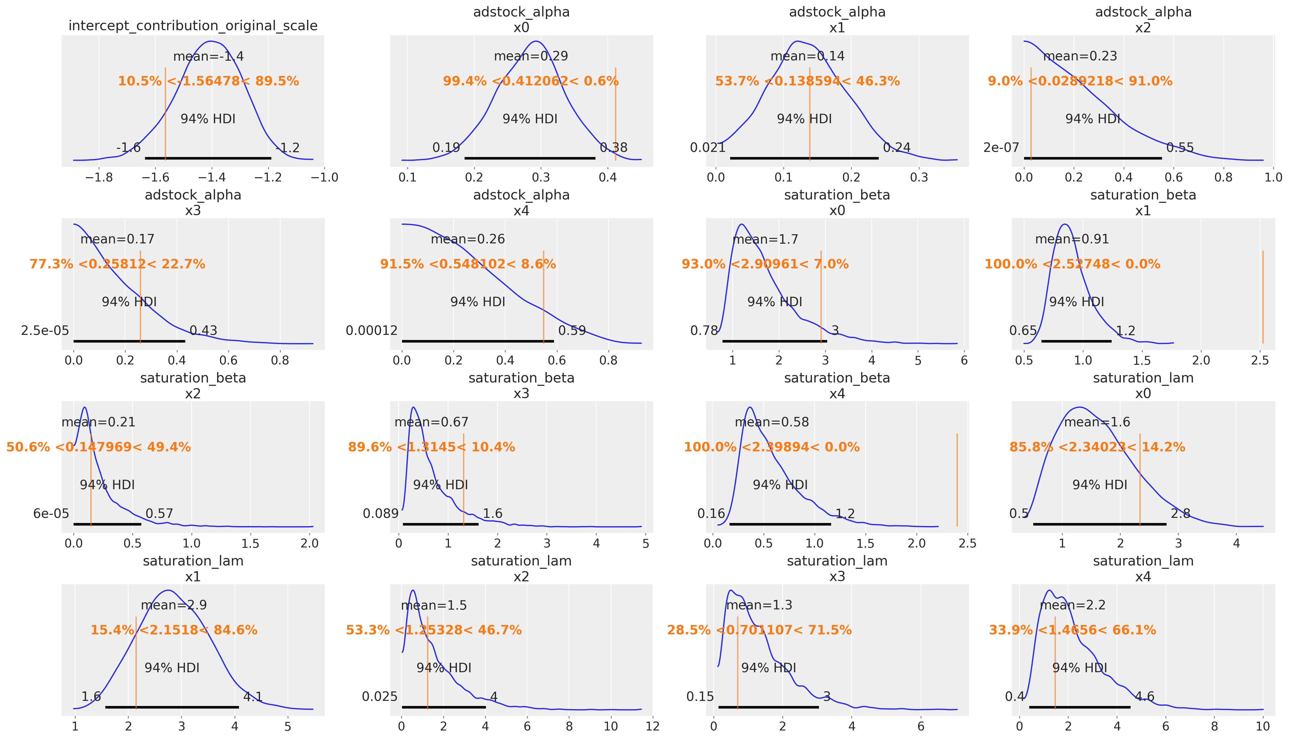
Model Parameters

We use az.plot_posterior with ref_val to overlay the true parameter values (vertical reference lines) on the posterior densities. If the reference lines fall within the bulk of each posterior distribution, the parameter recovery is successful.

az.plot_posterior(
    mmm.idata,
    var_names=[
        "intercept_contribution_original_scale",
        "adstock_alpha",
        "saturation_beta",
        "saturation_lam",
    ],
    ref_val={
        "intercept_contribution_original_scale": [{"ref_val": intercept_true}],
        "adstock_alpha": [
            {"channel": f"x{i}", "ref_val": adstock_alpha_true[i]}
            for i in range(n_channels)
        ],
        "saturation_beta": [
            {"channel": f"x{i}", "ref_val": saturation_beta_true[i]}
            for i in range(n_channels)
        ],
        "saturation_lam": [
            {"channel": f"x{i}", "ref_val": saturation_lam_true[i]}
            for i in range(n_channels)
        ],
    },
    figsize=(21, 12),
);

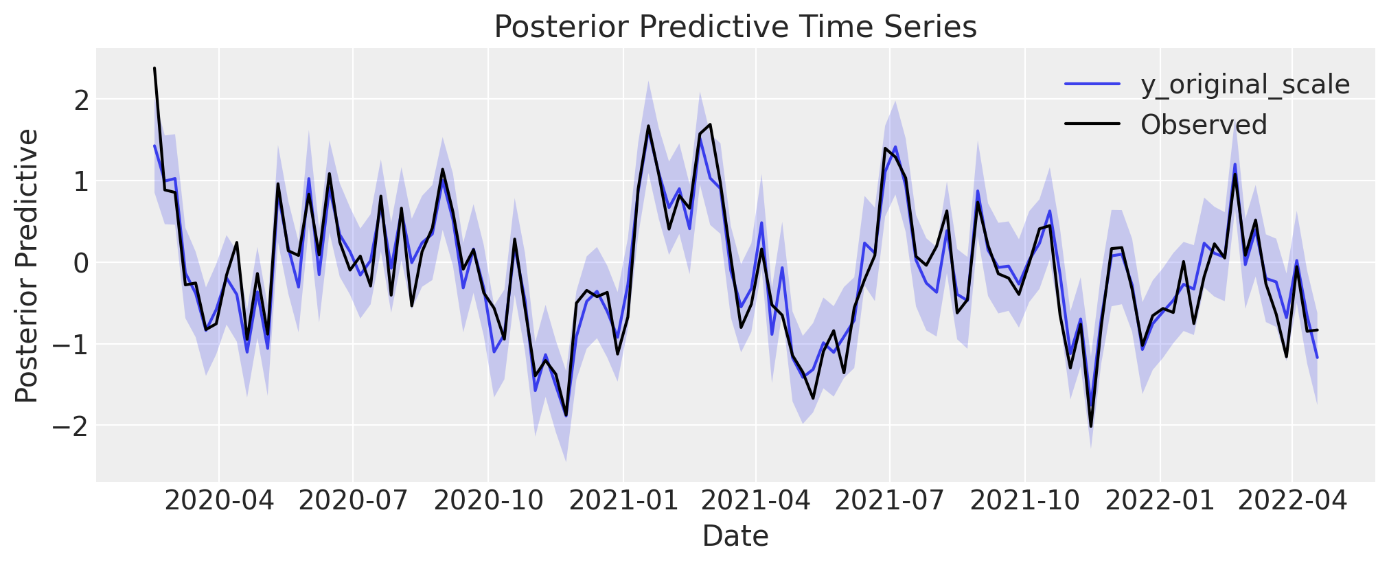
Posterior Predictive

The posterior predictive distribution should tightly envelop the observed (synthetic) time series. A good fit here confirms the model can reproduce the overall signal, including trends and seasonality.

fig, axes = mmm.plot.posterior_predictive(var=["y_original_scale"], hdi_prob=0.94)
sns.lineplot(
    data=mmm_df, x="date", y="y_obs", color="black", label="Observed", ax=axes[0][0]
);

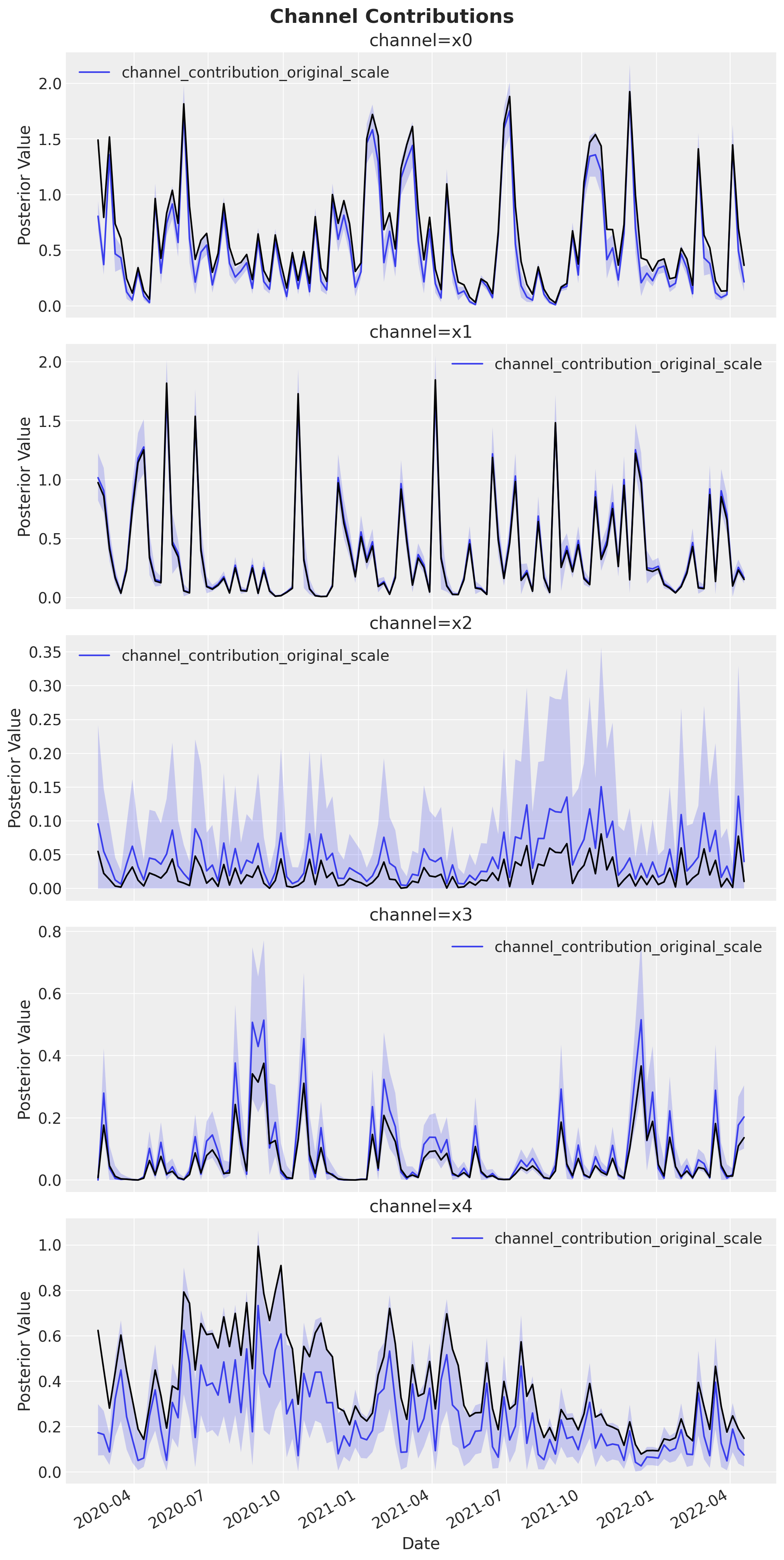
Channel Contributions

We compare the estimated channel contribution curves (with uncertainty bands) against the known true contributions (black lines). Good overlap between the posterior estimates and the ground-truth curves validates that the model correctly decomposes the total target signal into individual channel effects.

fig, axes = mmm.plot.contributions_over_time(
    var=["channel_contribution_original_scale"], hdi_prob=0.94
)

axes = axes.flatten()

for i, channel in enumerate(coords["channel"]):
    channel_contribution_observed = (
        idata_obs["prior"]["channel_contribution_original_scale"]
        .sel(chain=0, draw=0)
        .sel(channel=channel)
        .to_numpy()[l_max:]
    )

    sns.lineplot(
        data=mmm_df,
        x="date",
        y=channel_contribution_observed,
        color="black",
        ax=axes[i],
    )

fig.autofmt_xdate()
fig.suptitle("Channel Contributions", fontsize=18, fontweight="bold");

%load_ext watermark
%watermark -n -u -v -iv -w

Last updated: Thu, 12 Feb 2026

Python implementation: CPython
Python version       : 3.13.12
IPython version      : 9.10.0

arviz         : 0.23.4
matplotlib    : 3.10.8
numpy         : 2.3.5
pandas        : 2.3.3
pymc          : 5.27.1
pymc_extras   : 0.8.0
pymc_marketing: 0.18.0
pytensor      : 2.37.0
seaborn       : 0.13.2

Watermark: 2.6.0